Building an Experiment

Borealis has an extensive set of features and this means that experiments can be designed to be very simple or very complex. To help organize writing of experiments, we’ve designed the system so that experiments can be broken into smaller components, called slices, that interface together with other components to perform desired functionality. An experiment can have a single slice or several working together, depending on the complexity.

Each slice contains the information needed about a specific pulse sequence to run. The parameters of a slice contain features such as pulse sequence, frequency, fundamental time lag spacing, etc. These are the parameters that researchers will be familiar with. Each slice can be an experiment on its own, or can be just a piece of a larger experiment.

• New Experimental Capabilities
  • Simultaneous Full Field-of-View Imaging
  • Bistatic Experiments

Introduction to Borealis Slices

Slices are software objects made for the Borealis system that allow easy integration of multiple modes into a single experiment. Each slice could be an experiment on its own, and averaged data products are produced from each slice individually. Slices can be used to create separate frequency channels, separate pulse sequences, separate beam scanning order, etc. that can run simultaneously.

A slice is defined using a python dictionary with the necessary slice keys. For a complete list of keys that can be used in a slice, see Slice Keys.

The other necessary part of an experiment is specifying how slices will interface with each other. Interfacing in this case refers to how these two components are meant to be run. To understand the interfacing, lets first understand the basic building blocks of a SuperDARN experiment. These are:

Sequence

Made up of pulses of a specific duration (pulse length) with a specified fundamental (tau) spacing, at a specified frequency, and with a specified receive time (duration) following the transmission (to gather information from the number of ranges specified). Researchers might be familiar with a common SuperDARN 7 or 8 pulse sequence design. The sequence definition here is the time to transmit one sequence and the time for receiving echoes from that sequence.

Averaging period

A time duration where the sequences are repeated to gather enough information to average and reduce the effect of spurious emissions on the data. These are defined by either a number of sequences, or a length of time during which as many sequences as possible are transmitted. For example, researchers may be familiar with the standard 3 second averaging period in which ~30 pulse sequences are sent out and received in a single beam direction.

Scan

A time where the averaging periods are repeated, traditionally to look in different beam directions with each averaging period. A scan is defined by the number of beams or integration times. Researchers may be familiar with the standard 1-minute 16-beam scan from East to West, or West to East, depending upon the radar.

Interfacing Types Between Slices

src.experiment_prototype.experiment_prototype.interface_types = ('SCAN', 'AVEPERIOD', 'SEQUENCE', 'CONCURRENT')

Interfacing in this case refers to how two or more slices are meant to be run together. The following types of interfacing between slices are possible, arranged from highest level of experiment building-block to the lowest level:

1. SCAN

   The scan-by-scan interfacing allows for slices to run a scan of one slice, followed by a scan of the second. The scan mode of interfacing typically means that the slice will cycle through all of its beams before switching to another slice.

   There are no requirements for slices interfaced in this manner.

2. AVEPERIOD

   This type of interfacing allows for one slice to run its averaging period (also known as integration time or integration period), before switching to another slice’s averaging period. This type of interface effectively creates an interleaving scan where the scans for multiple slices are run ‘at the same time’, by interleaving the averaging periods.

   Slices which are interfaced in this manner must share:

   • the same SCANBOUND value.

3. SEQUENCE

   Sequence interfacing allows for pulse sequences defined in the slices to alternate between each other within a single averaging period. It’s important to note that data from a single slice is averaged only with other data from that slice. So in this case, the averaging period is running two slices and can produce two averaged datasets, but the sequences within the averaging period are interleaved.

   Slices which are interfaced in this manner must share:

   • the same SCANBOUND value.

   • the same INTT or INTN value.

   • the same BEAM_ORDER length (scan length).

   • the same TXCTRFREQ value.

   • the same RXCTRFREQ value.

4. CONCURRENT

   Concurrent interfacing allows for pulse sequences to be run together concurrently. Slices will have their pulse sequences summed together so that the data transmits at the same time. For example, slices of different frequencies can be mixed simultaneously, and slices of different pulse sequences can also run together at the cost of having more blanked samples. When slices are interfaced in this way the radar is truly transmitting and receiving the slices simultaneously.

   Slices which are interfaced in this manner must share:

   • the same SCANBOUND value.

   • the same INTT or INTN value.

   • the same BEAM_ORDER length (scan length).

   • the same TXCTRFREQ value.

   • the same RXCTRFREQ value.

   • the same DECIMATION_SCHEME.

Slice Interfacing Examples

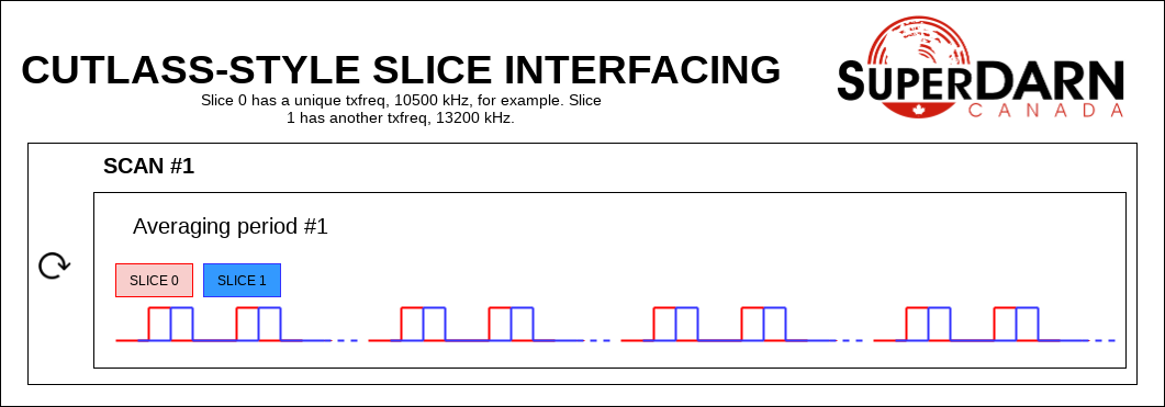
Let’s look at some examples of common experiments that can easily be separated into multiple slices. In these examples, the ⟳ means that the averaging period is repeated multiple times in a scan, and the different slices are colour coded.

In a CUTLASS-style experiment, the pulse in the sequence is actually two pulses of differing transmit frequency. This is a ‘quasi’-simultaneous multi-frequency experiment where the frequency changes in the middle of the pulse. To build this experiment, two slices can be CONCURRENT interfaced. The pulses from both slices are combined into a single set of transmitted samples for that sequence and samples received from those sequences are used for both slices (filtering the raw data separates the frequencies).

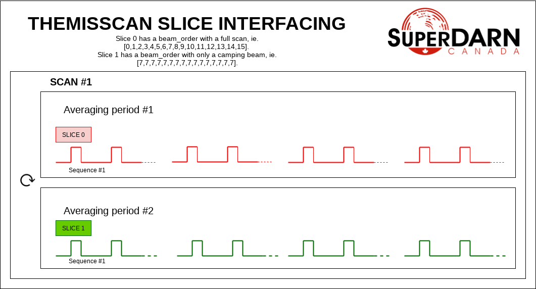
In a themisscan experiment, a single beam is interleaved with a full scan. The beam_order can be unique to different slices, and these slices could be AVEPERIOD interfaced to separate the camping beam data from the full scan, if desired. With AVEPERIOD interfacing, one averaging period of one slice will be followed by an averaging period of another, and so on. The averaging periods are interleaved. The resulting experiment runs beams 0, 7, 1, 7, etc.

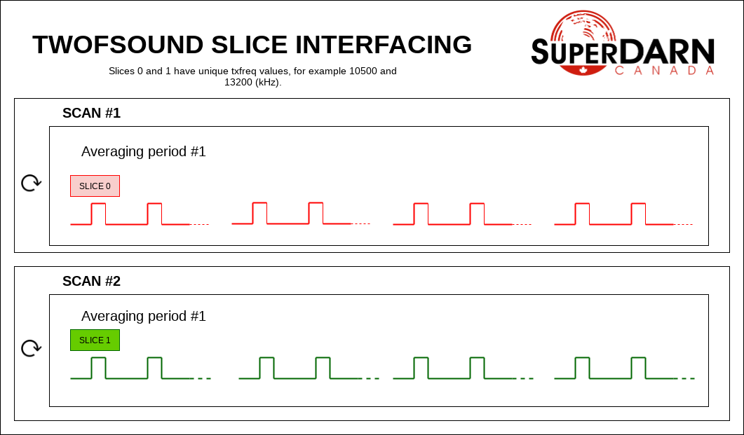
In a twofsound experiment, a full scan of one frequency is followed by a full scan of another frequency. The txfreq are unique between the slices. In this experiment, the slices are SCAN interfaced. A full scan of slice 0 runs followed by a full scan of slice 1, and then the process repeats.

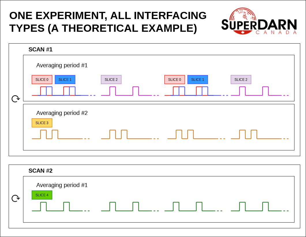
Here’s a theoretical example showing all types of interfacing. In this example, slices 0 and 1 are CONCURRENT interfaced. Slices 0 and 2 are SEQUENCE interfaced (Note that when slices 0 and 2 are SEQUENCE interfaced, that automatically implies that slices 1 and 2 are also SEQUENCE interfaced). Slices 0 and 3 are AVEPERIOD interfaced (again, note that this implies that slices 1 and 3 are AVEPERIOD interfaced, additionally that slices 2 and 3 are AVEPERIOD interfaced). Slices 0 and 4 are SCAN interfaced (finally, to really drive home this point, this implies that slices 1 and 4 are SCAN interfaced, slices 2 and 4 are SCAN interfaced, and slices 3 and 4 are SCAN interfaced).

Writing an Experiment

All experiments must be written as their own class and must be built off of the built-in ExperimentPrototype class.

This means the ExperimentPrototype class must be imported at the start of the experiment file

from experiment_prototype.experiment_prototype import ExperimentPrototype

Please name the class within the experiment file in a similar fashion to the file, as the class name is written to the datasets produced.

The experiment has the following experiment-wide attributes:

cpid required

The only experiment-wide attribute that is required to be set by the user when initializing is the CPID, or control program identifier. This must be unique to the experiment. You will need to request this from your institution’s radar operator. You should clearly document the name of the experiment and some operating details that correspond to the CPID. Please see this SuperDARN Canada webpage for more information, and to see lists of CPIDs that already exist.

output_rx_rate defaults

The sampling rate of the output data. The default is 10.0e3/3 Hz, or 3.333 kHz.

rx_bandwidth defaults

The sampling rate of the USRPs (before decimation). The default is 5.0e6 Hz, or 5 MHz.

tx_bandwidth defaults

The output sampling rate of the transmitted signal. The default is 5.0e6 Hz, or 5 MHz.

comment_string defaults

A comment string describing the experiment. It is highly encouraged to provide some description of the experiment for the output data files. The default is ‘’, or an empty string.

Below is an example of properly inheriting the prototype class and defining your own experiment:

class MyClass(ExperimentPrototype):

    def __init__(self):
        cpid = 123123  # this must be a unique id for your control program.
        super().__init__(cpid,
            comment_string='My experiment explanation')

The experiment handler will create an instance of your experiment when your experiment is scheduled to start running. Your class is a child class of ExperimentPrototype and because of this, the parent class needs to be instantiated when the experiment is instantiated. This is important because the experiment_handler will build the scans required by your class in a way that is easily readable and iterable by the radar control program. This is done by methods that are set up in the ExperimentPrototype parent class.

The next step is to add slices to your experiment. An experiment is defined by the slices in the class, and how the slices interface. As mentioned above, slices are just python dictionaries, with a preset list of keys available to define your experiment. The keys that can be used in the slice dictionary are described below.

Slice Keys

class src.experiment_prototype.experiment_slice.ExperimentSlice

These are the keys that are set by the user when initializing a slice. Some are required, some can be defaulted, and some are set by the experiment and are read-only.

Slice Keys Required by the User

beam_angle required

list of beam directions, in degrees off azimuth. Positive is E of N. The beam_angle list length = number of beams. Traditionally beams have been 3.24 degrees separated but we don’t refer to them as beam -19.64 degrees, we refer as beam 1, beam 2. Beam 0 will be the 0th element in the list, beam 1 will be the 1st, etc. These beam numbers are needed to write the [rx|tx]_beam_order list. This is like a mapping of beam number (list index) to beam direction off boresight.

clrfrqrange required or freq required

range for clear frequency search, should be a list of length = 2, [min_freq, max_freq] in kHz. Not currently supported.

first_range required

first range gate, in km

freq required or clrfrqrange required

transmit/receive frequency, in kHz. Note if you specify clrfrqrange it won’t be used.

intt required or intn required

duration of an averaging period (integration), in ms. (maximum)

intn required or intt required

number of averages to make a single averaging period (integration), only used if intt = None

num_ranges required

Number of range gates to receive for. Range gate time is equal to pulse_len and range gate distance is the range_sep, calculated from pulse_len.

pulse_len required

length of pulse in us. Range gate size is also determined by this.

pulse_sequence required

The pulse sequence timing, given in quantities of tau_spacing, for example normalscan = [0, 14, 22, 24, 27, 31, 42, 43].

rx_beam_order required

beam numbers written in order of preference, one element in this list corresponds to one averaging period. Can have lists within the list, resulting in multiple beams running simultaneously in the averaging period, so imaging. A beam number of 0 in this list gives us the direction of the 0th element in the beam_angle list. It is up to the writer to ensure their beam pattern makes sense. Typically rx_beam_order is just in order (scanning W to E or E to W), ie. [0, 1, 2, 3, 4, 5, 6, 7, 8, 9, 10, 11, 12, 13, 14, 15]. You can list numbers multiple times in the rx_beam_order list, for example [0, 1, 1, 2, 1] or use multiple beam numbers in a single averaging period (example [[0, 1], [3, 4]], which would trigger an imaging integration. When we do imaging we will still have to quantize the directions we are looking in to certain beam directions. It is up to the user to ensure that this field works well with the specified tx_beam_order or tx_antenna_pattern.

rxonly read-only

A boolean flag to indicate that the slice doesn’t transmit, only receives.

tau_spacing required

multi-pulse increment (mpinc) in us, Defines minimum space between pulses.

Defaultable Slice Keys

acf defaults

flag for rawacf generation. The default is False. If True, the following fields are also used: - averaging_method (default ‘mean’) - xcf (default True if acf is True) - acfint (default True if acf is True) - lagtable (default built based on all possible pulse combos) - range_sep (will be built by pulse_len to verify any provided value)

acfint defaults

flag for interferometer autocorrelation data. The default is True if acf is True, otherwise False.

align_sequences defaults

flag for aligning the start of the first pulse in each sequence to tenths of a second. Default False.

averaging_method defaults

a string defining the type of averaging to be done. Current methods are ‘mean’ or ‘median’. The default is ‘mean’.

comment defaults

a comment string that will be placed in the borealis files describing the slice. Defaults to empty string.

lag_table defaults

used in acf calculations. It is a list of lags. Example of a lag: [24, 27] from 8-pulse normalscan. This defaults to a lagtable built by the pulse sequence provided. All combinations of pulses will be calculated, with both the first pulses and last pulses used for lag-0.

pulse_phase_offset defaults

a handle to a function that will be used to generate one phase per each pulse in the sequence. If a function is supplied, the beam iterator, sequence number, and number of pulses in the sequence are passed as arguments that can be used in this function. The default is None if no function handle is supplied.

encode_fn(beam_iter, sequence_num, num_pulses):

return np.ones(size=(num_pulses))

The return value must be numpy array of num_pulses in size. The result is a single phase shift for each pulse, in degrees.

Result is expected to be real and in degrees and will be converted to complex radians.

range_sep defaults

a calculated value from pulse_len. If already set, it will be overwritten to be the correct value determined by the pulse_len. Used for acfs. This is the range gate separation, in the radial direction (away from the radar), in km.

rxctrfreq defaults

Center frequency, in kHz, used to mix to baseband. Since this requires tuning time to set, it is the user’s responsibility to ensure that the re-tuning time does not detract from the experiment implementation. Tuning time is set in the usrp_driver.cpp script and changes to the time will require recompiling of the code.

rx_intf_antennas defaults

The antennas to receive on in interferometer array, default is all antennas given max number from config.

rx_main_antennas defaults

The antennas to receive on in main array, default is all antennas given max number from config.

rx_antenna_pattern defaults

Experiment-defined function which returns a complex weighting factor of magnitude <= 1 for each beam direction scanned in the experiment. The return value of the function must be an array of size [beam_angle, antenna_num]. This function allows for custom beamforming of the receive antennas for borealis processing of antenna iq to rawacf.

scanbound defaults

A list of seconds past the minute for averaging periods in a scan to align to. Defaults to None, not required. If one slice in an experiment has a scanbound, they all must.

seqoffset defaults

offset in us that this slice’s sequence will begin at, after the start of the sequence. This is intended for CONCURRENT interfacing, when you want multiple slice’s pulses in one sequence you can offset one slice’s sequence from the other by a certain time value so as to not run both frequencies in the same pulse, etc. Default is 0 offset.

txctrfreq defaults

Center frequency, in kHz, for the USRP to mix the samples with. Since this requires tuning time to set, it is the user’s responsibility to ensure that the re-tuning time does not detract from the experiment implementation. Tuning time is set in the usrp_driver.cpp script and changes to the time will require recompiling of the code.

tx_antennas defaults

The antennas to transmit on, default is all main antennas given max number from config.

tx_antenna_pattern defaults

experiment-defined function which returns a complex weighting factor of magnitude <= 1 for each tx antenna used in the experiment. The return value of the function must be an array of size [num_beams, main_antenna_count] with all elements having magnitude <= 1. This function is analogous to the beam_angle field in that it defines the transmission pattern for the array, and the tx_beam_order field specifies which “beam” to use in a given averaging period.

tx_beam_order defaults, but required if tx_antenna_pattern given

beam numbers written in order of preference, one element in this list corresponds to one averaging period. A beam number of 0 in this list gives us the direction of the 0th element in the beam_angle list. It is up to the writer to ensure their beam pattern makes sense. Typically tx_beam_order is just in order (scanning W to E or E to W, i.e. [0, 1, 2, 3, 4, 5, 6, 7, 8, 9, 10, 11, 12, 13, 14, 15]. You can list numbers multiple times in the tx_beam_order list, for example [0, 1, 1, 2, 1], but unlike rx_beam_order, you CANNOT use multiple beam numbers in a single averaging period. In other words, this field MUST be a list of integers, as opposed to rx_beam_order, which can be a list of lists of integers. The length of this list must be equal to the length of the rx_beam_order list. If tx_antenna_pattern is given, the items in tx_beam_order specify which row of the return from tx_antenna_pattern to use to beamform a given transmission. Default is None, i.e. rxonly slice.

wait_for_first_scanbound defaults

A boolean flag to determine when an experiment starts running. True (default) means an experiment will wait until the first averaging period in a scan to start transmitting. False means an experiment will not wait for the first averaging period, but will instead start transmitting at the nearest averaging period. Note: for multi-slice experiments, the first slice is the only one impacted by this parameter.

xcf defaults

flag for cross-correlation data. The default is True if acf is True, otherwise False.

Read-only Slice Keys

clrfrqflag read-only

A boolean flag to indicate that a clear frequency search will be done. Not currently supported.

cpid read-only

The ID of the experiment, consistent with existing radar control programs. This is actually an experiment-wide attribute but is stored within the slice as well. This is provided by the user but not within the slice, instead when the experiment is initialized.

slice_id read-only

The ID of this slice object. An experiment can have multiple slices. This is not set by the user but instead set by the experiment when the slice is added. Each slice id within an experiment is unique. When experiments start, the first slice_id will be 0 and incremented from there.

slice_interfacing read-only

A dictionary of slice_id : interface_type for each sibling slice in the experiment at any given time.

Experiment Example

An example of adding a slice to your experiment is as follows:

tau_spacing = 2100
first_slice = {  # slice_id will be 0, there is only one slice.
    "pulse_sequence": [0, 9, 12, 20, 22, 26, 27],  # the common 7-pulse sequence in SDARN
    "tau_spacing": tau_spacing,  # us
    "pulse_len": 300,  # us
    "num_ranges": 75,  # range gates
    "first_range": 180,  # first range gate, in km
    "intt": 3500,  # duration of an integration, in ms
    "beam_angle": [-24.3, -21.06, -17.82, -14.58, -11.34, -8.1, -4.86, -1.62, 1.62, 4.86, 8.1, 11.34,
    14.58, 21.06, 24.3],  # 16 beams, separated by 3.24 degrees
    "rx_beam_order": [15, 14, 13, 12, 11, 10, 9, 8, 7, 6, 5, 4, 3, 2, 1, 0],
    "tx_beam_order": [15, 14, 13, 12, 11, 10, 9, 8, 7, 6, 5, 4, 3, 2, 1, 0],
    "scanbound": [i * 3.5 for i in range(len(beams_to_use))], #1 min scan
    "freq" : 10500, #kHz
    "acf": True,
    "xcf": True,  # cross-correlation processing
    "acfint": True,  # interferometer acfs
    "wait_for_first_scanbound": False,
}

self.add_slice(first_slice)

This slice would be assigned with slice_id = 0 if it’s the first slice added to the experiment. The experiment could also add another slice:

second_slice = copy.deepcopy(first_slice)
second_slice['freq'] = 13200 # kHz
second_slice['comment'] = 'This is my second slice, it has a different frequency.'

self.add_slice(second_slice, interfacing_dict={0: 'SCAN'})

Notice that you must specify interfacing to an existing slice when you add a second or greater order slice to the experiment. To see the types of interfacing that can be used, see the above section Interfacing Types Between Slices.

This experiment is very similar to the twofsound experiment. To see examples of common experiments, look at Experiments.

Checking Your Experiment for Errors

An experiment testing script experiment_unittests.py has been written to check experiments for errors and ensure the operation of experiment checking source code. This suite of tests can be run by the following command:

python3 BOREALISPATH/tests/experiments/experiment_unittests.py

This will test all experiments within the borealis_experiments directory, and run all exception-checking unit tests within the testing_archive directory of the experiments directory. At the end, the results of all tests will be summarized, showing how many tests passed and failed.

This testing script can also be used to check specific experiments are written correctly. To do this, ensure your experiment is in the src/borealis_experiments directory and run the following command:

python3 BOREALISPATH/tests/experiments/experiment_unittests.py --experiment [EXPERIMENT_NAME]

where EXPERIMENT_NAME is the module name of your experiment. If there are any errors while checking your experiment, the test will fail and the exception will describe the error.

• Experiment Unittests