Walkthrough of the Borealis Processing Chain¶

Filtering¶

Filtering Stages¶

The Borealis processing chain uses a staged-filter approach with staged downsampling, allowing for multi-frequency filtering in real time. Using numpy arrays and array operations, the broadband input spectrum received from the N200 devices can be filtered simultaneously into multiple datasets centered on different frequencies. The data is first run through frequency-translating bandpass filters to create multiple baseband output spectra, one for each filter frequency. This is done in one algorithm using the modified Frerking method described in Section Modified Frerking Method and at Another representation of Frerking’s method.

Following the bandpass-mixing filter, three stages of lowpass filtering and downsampling are done. These stages are identical for all mixing frequencies.

As with most aspects of the Borealis system, there is freedom for customization of the filtering stages. The filtering stages are stored in a DecimationScheme class which is stored in the experiment file. If no DecimationScheme is provided, a default is used. Most Borealis experiments use this default scheme, which will be described in more detail below in Section Default DecimationScheme.

A Jupyter notebook is included with the Borealis software for visualization and testing of filtering schemes, using the filtering methods that run when a Borealis radar operates. This notebook can be found at $BOREALISPATH/tests/dsp_testing/filters.ipynb.

Default DecimationScheme¶

The default DecimationScheme for Borealis uses a 4-stage filter and downsampling to reduce the data rate from 5 MHz to 3.333 kHz. The input sampling rate, downsampling rate, and output sampling rate are shown for each stage in the table below.

Filter Stage	Input Rate	Downsampling Rate	Output Rate	Number of Taps
0	5 MHz	10	500 kHz	661
1	500 kHz	5	100 kHz	127
2	100 kHz	6	16.667 kHz	27
3	16.667 kHz	5	3.333 kHz	4

For a typical sequence of normalscan data, the input data to the first filter stage contains 451500 complex data samples for each antenna. After the first stage, this has been reduced to 45084 samples per antenna, but if multiple frequencies are being selected, there will be one copy of ( $num\_antennas$ , 45084) for each frequency. After the second stage, the number of samples is reduced from 45084 to 8992. The next stage reduces it again to 1495 samples. Lastly, the final stage reduces the data length to 299 samples. The number of samples in and out of each stage does not exactly correspond to the downsampling rate; this will be explained shortly, as a result of the filtering technique.

All Borealis signal processing is done in the time domain. The following figures illustrate the process for a hypothetical 10-sample dataset and 3-tap filter.

Figure 1 shows the dataset $x$ and the filter taps $h$ . For all stages of filtering, $x$ is much longer than $h$ , by three to four orders of magnitude.

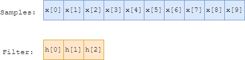
Figure 1: Graphical depiction of a data sequence and filter sequence¶

Figure 2 shows the process of linear convolution of $h$ with $x$ . The sequence $h$ is flipped, then slid along $x$ and multiplied element-wise. At each position, the sum of the element-wise multiplication is the output sample, call it $y[n]$ . We can see that the sequence $y$ will be longer than $x$ . The length of $y$ is equal to the length of $h$ plus the length of $x$ , minus one. However, the samples of $y$ for which $h$ was “hanging off” of $x$ exhibit undesirable edge effects. In Borealis, these samples are dropped. Thus, the first sample of $y$ corresponds to the third iteration shown in Figure 2, and similarly the last sample kept is the third-last sample in the convolution. In general, the number of dropped samples at each the start and end of the convolution is equal to the filter length minus one. The dropping of samples can be seen in Figure 3.

To speed up the processing, downsampling in Borealis is done in the convolution step. This is done by sliding $h$ in steps of the downsampling rate, as shown in Figure 3. This is mathematically equivalent to taking the linear convolution then downsampling, but is computationally faster.

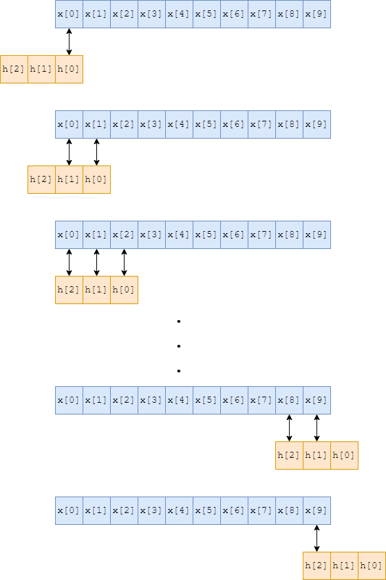
Figure 2: Linear convolution of two sequences¶

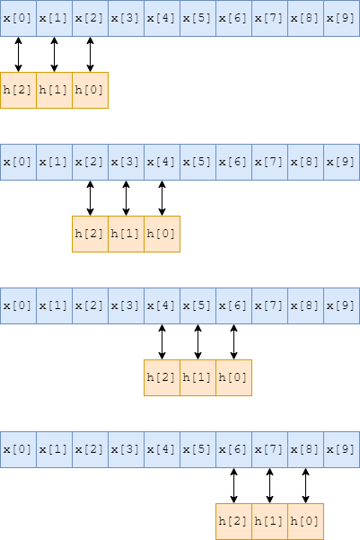
Downsampled convolution with edge effects discarded

Figure 3: Linear convolution and downsampling, with filter roll-off samples dropped¶

Modified Frerking Method¶

The Frerking method is used to extract a narrow frequency from a wideband spectrum. The method is identical to the traditional multi-step approach of mixing an incoming signal with an oscillator to bring the desired frequency to baseband, then running it through a low-pass filter.

Mixing a signal with an oscillator is just multiplying the signal with the oscillator value as the signals are coming in. Since we gather complex samples, we use a complex oscillator (a complex exponential instead of a cosine). To accomplish this in one (actually two) step(s), the complex exponential is multiplied into the filter coefficients. Then, the wideband samples are passed through the filter, which simultaneously mixes the samples and low-pass filters them. However, there is still one more detail to resolve (the second step). In an analog system, the phase of the oscillator changes over time, as might be obvious from the name “oscillator”. So, as samples arrive, they are multiplied by the oscillator value at the moment they arrive. However, with Borealis we are mixing with the filter sequence, rather than the input samples (less multiplications). We mix the oscillator with the filter once, then run the input samples through the filter. The top curve in Figure 4 depicts the numerical oscillator sequence that gets mixed with the filter sequence. As the filter sequence “slides” along the input samples, the phase is not consistent with an equivalent analog mixing system.

As the filter “slides” along the samples, we are effectively getting a different window of the input samples. The curves in Figure 4 depict the analog mixer sequence for each windowed view of the input samples (the legend corresponds to the output sample number). In Borealis, there is only one mixer sequence - the top curve. As we apply the filter and “slide” along the input samples, we then have a phase difference between Borealis and its equivalent analog system. This difference is fairly simple to correct. If the oscillator has phase ${\phi}_0 = 0$ when it mixes with the zeroth sample, then it will have phase $\phi_1 = 2\pi\frac{f_o}{F_s}$ when it mixes with the first sample, $\phi_2 = 2\pi\frac{f_o}{F_s}2$ when it mixes with the second sample, and so on. The general formula is $\phi_k = 2\pi\frac{f_o}{F_s}k$ , where $f_o$ is the oscillator frequency, $F_s$ is the data sampling rate, and $k$ is the index of the newest sample. Borealis applies this correction after applying the filter and decimating, to reduce the number of mathematical operations. So, for a downsampling rate of $R$ , the phase correction for sample $k$ after downsampling is $\phi_k = 2\pi\frac{f_o}{F_s}Rk$ .

Windowed view of oscillator mixing sequence

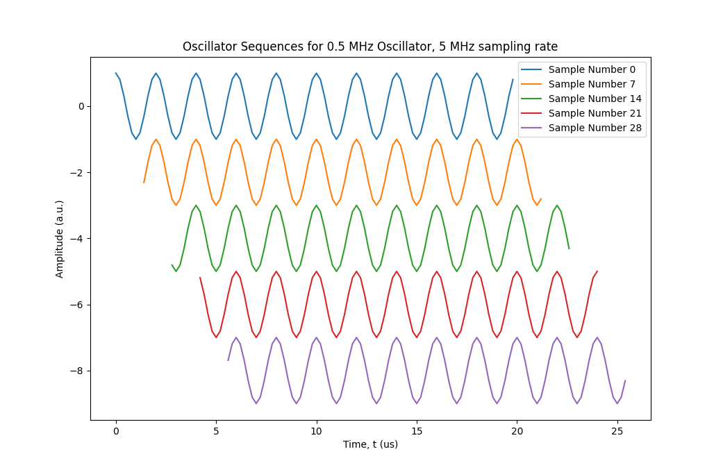
Figure 4: Oscillator sequence evolution with sample number¶

Standard Filters¶

As mentioned previously, Borealis uses a four-stage filter approach with staged downsampling. These filters are shown in Figures 5, 6, 7, and 8.

The first stage of filtering uses the Frerking method to simultaneously filter and mix to baseband. The passband center frequency of the filter is configurable, and changes automatically to match the frequency used in the experiment. Figure 5 shows the first stage of filter, with a passband centered around 0.5 MHz. Figure 9 shows the same stage, but for a different center frequency of 2.0 MHz. After this stage, the samples are decimated by a factor of 10 then passed through the lowpass filter shown in Figure 6. The data is then decimated again by a factor of 5, then passed through the filter shown in Figure 7. Another decimation by a factor of 6, passed through the filter in Figure 7, then a final decimation by a rate of 5 yields the antennas IQ dataset.

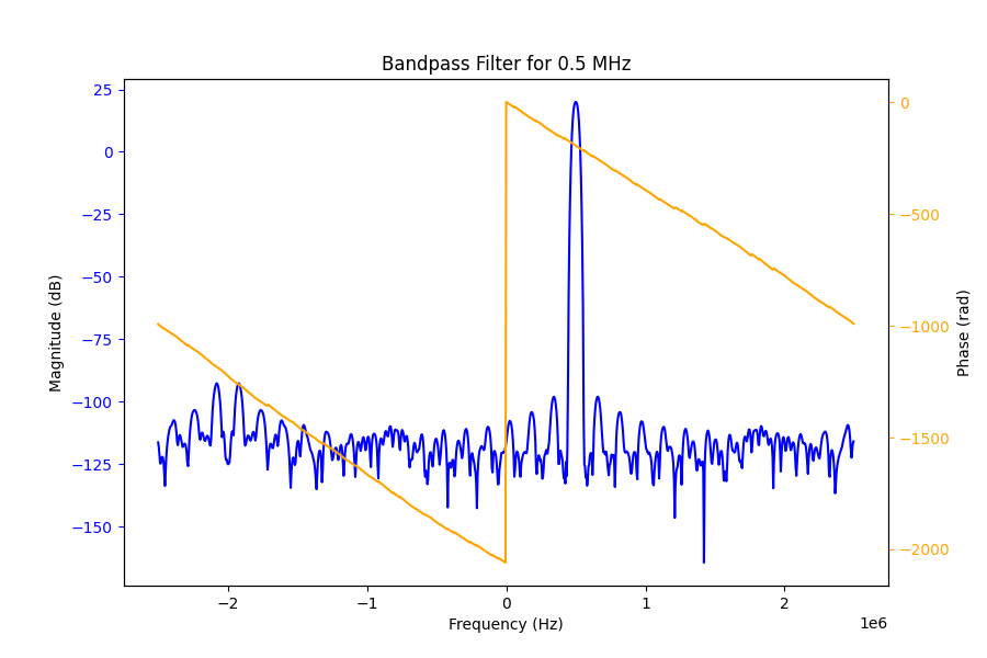
Figure 5: 0.5 MHz Bandpass Filter Frequency Response¶

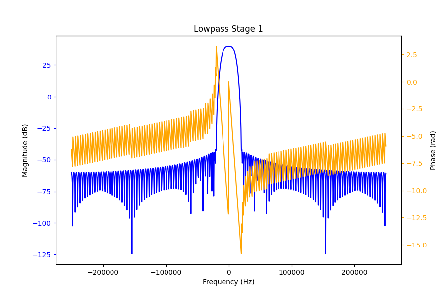
Figure 6: Stage 1 Lowpass Filter Frequency Response¶

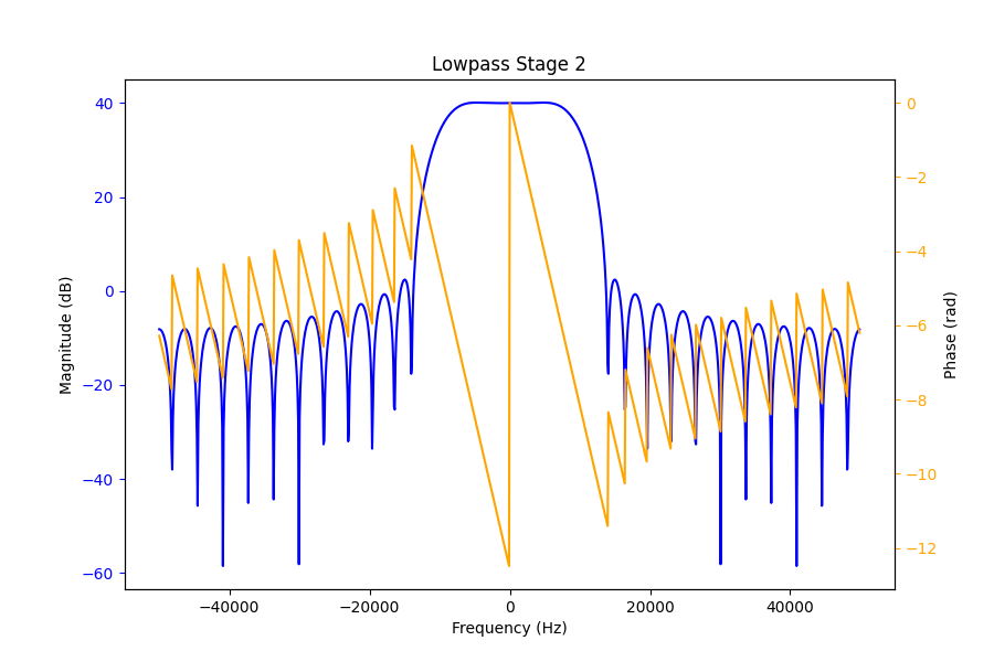
Figure 7: Stage 2 Lowpass Filter Frequency Response¶

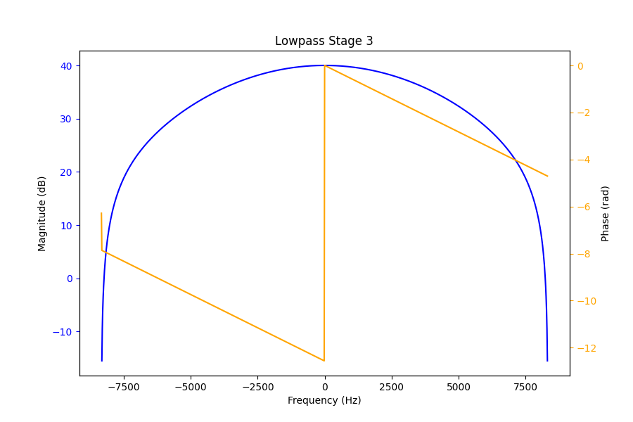
Figure 8: Stage 3 Lowpass Filter Frequency Response¶

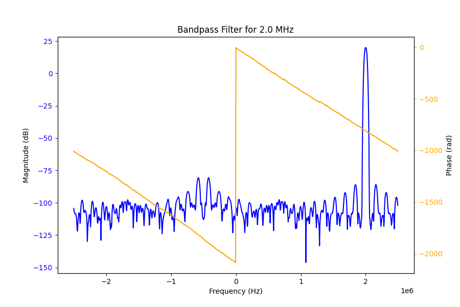
Figure 9: 2.0 MHz Bandpass Filter Frequency Response¶

One thing to note is the sampling bandwidth of the data directly from the USRPs. Borealis specifies a receive frequency band to the USRPs, and all data lies within that band. Ordinarily, this band is defined by a bandwidth of 5 MHz centered around 12 MHz, for a total range of 9.5-14.5 MHz. If one were to plot the FFT of the data, the FFT frequencies will take the range of (-2.5 MHz, 2.5 MHz). If the transmitted signal was at 10.5 MHz, we then expect to see it in our received samples at (12.0 MHz - 10.5 MHz) = -1.5 MHz. Figure 10 shows exactly this situation.

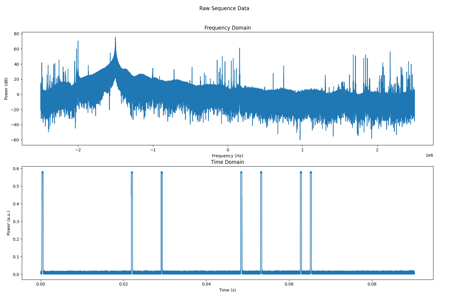
Time- and Frequency-domain representations of one sequence of received data at 10.5 MHz

Figure 10: Sample Sequence of raw data from 10.5 MHz transmitted signal¶

Beamforming¶

Beamforming in Borealis is relatively straightforward. Figure 11 illustrates the physical process, with the red antennas signifying the main array, the thick black line being the incoming plane wavefront, the parallel green lines indicating planar wavefronts at spacings of one wavelength, and the beam direction off of boresight shown by $\theta$ . For an incoming wave, we can see that it will hit the leftmost antenna (antenna 0) first, then antenna 1, antenna 2, and so forth, reaching antenna 15 last. Each antenna $n$ is going to measure a different phase of the wave, determined by its distance from the wavefront $d_n$ as shown in the figure. Due to $2\pi$ ambiguity, the relevant phase correction is the phase required to get from the antenna to the closest green line. The required phase shift can be calculated from the geometry of the diagram as

$\phi_n = \frac{d_n}{\lambda} 2\pi$

The filtered samples for a given antenna are multiplied by $\phi_n$ to correct their phase, then the samples for all antennas are summed together to yield one dataset for the linear array.

The final wrinkle to this process is in the positioning of the wavefront. In Borealis, it is assumed that the wavefront crosses the array axis at boresight, i.e. between antennas 7 and 8 where the dotted line intersects the array axis. This means that the distances $d_n$ for antennas 0 through 7 will be negative, since the wavefront will have passed them already. With this last detail considered, we can formulate the phase correction for a given beam angle $\theta$ . The result is

$d_n = (n-\frac{N}{2})L\sin(\theta)$

where $n$ is the antenna index, $N$ is the total number of antennas in the array, and $L$ is the uniform antenna spacing. Plugging this result into the previous formula yields a final formula of

$\phi_n = \left(\frac{L}{\lambda}(n-\frac{N}{2})\sin(\theta)\right) 2\pi$

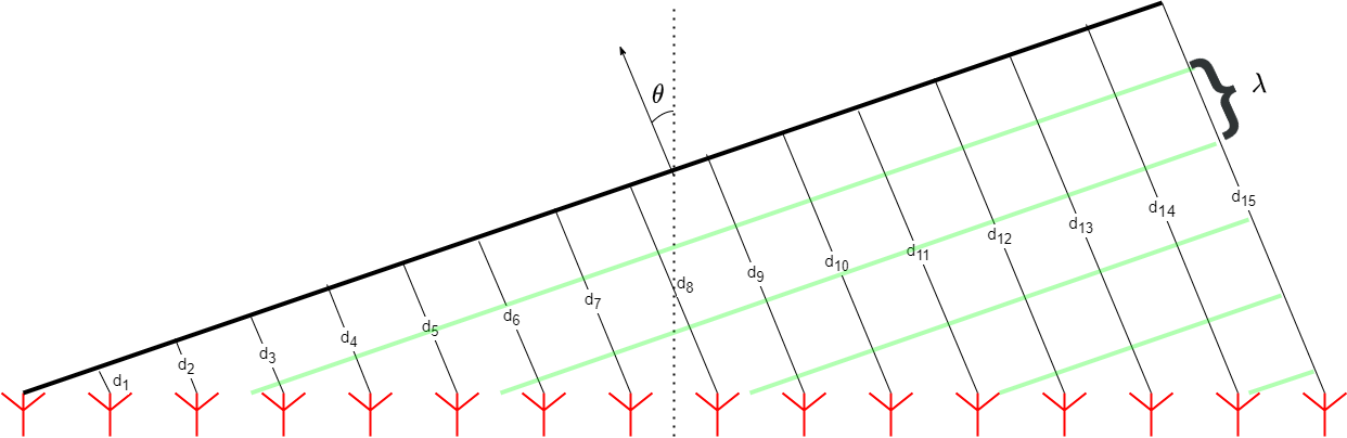
Figure 11: Geometry of 1-D phased array beamforming¶

Correlating¶

Once beamforming has been completed, the data is correlated to analyze the time evolution of signals scattered from the ionosphere. For each sequence, Borealis computes either one or three correlations. If only the main array is used, then the samples from that array are autocorrelated. If the interferometer is also used, the interferometer samples are autocorrelated, and the main and interferometer samples are cross-correlated. The process is the same for all correlations, and is described with the aid of Figure 12.

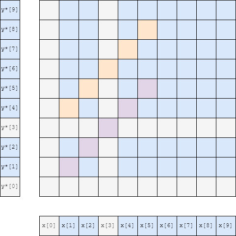
Figure 12: Correlation matrix with blanked samples removed and lag samples extracted¶

In Figure 12, the array samples are shown outside of the correlation, as the sequences $x$ and $y^*$ . For autocorrelation, $x = y$ , and for cross-correlation they are different, but always of the same length in Borealis. Grey samples are “blanked” samples, which occur when the radar is transmitting data. These samples are later disregarded, as the Borealis transmitters block ionospheric signals during transmit times. The 2-D matrix is the multiplication (outer product) of the two sequences. In this example, there are five range gates that we need data for, with the first range gate being one “sample” away from the radar, i.e. the range is half as far away as the distance light can travel in one unit of the sample spacing. The other useful time quantity required for this process is the lag spacing, denoted by $\tau$ . This is the common factor in all lag pairs of the data, which for this example is three samples, as pulses occur at $x[0]$ and $x[3]$ . We are interested in how the data is correlated in units of $\tau$ , for all ranges. To determine this, we correlate the data, and extract the correlations for all lags at all ranges. The purple samples in the correlation matrix are the correlations for lag-0 for the five ranges, with the closest range being $x[1]y^*[1]$ and the furthest range $x[5]y^*[5]$ . The orange samples represent the correlations for lag-1 for the same ranges. This data represents lag-1 as the samples are the correlation of data from $x$ and $y$ which occur $\tau$ seconds apart (three samples). Figure 13 shows the same style of diagram for a typical SuperDARN 7-pulse sequence, with 75 range gates, a tau spacing of 8 samples, and the first range occurring four samples after a pulse.

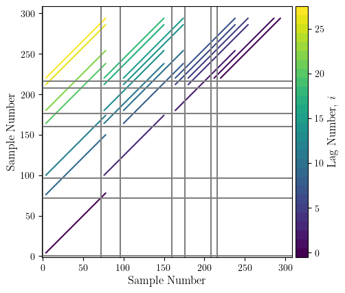
Figure 13: Borealis correlation matrix¶