Building an Experiment
Borealis has an extensive set of features and this means that experiments can be designed to be very simple or very complex. To help organize writing of experiments, we’ve designed the system so that experiments can be broken into smaller components, called slices, that interface together with other components to perform desired functionality. An experiment can have a single slice or several working together, depending on the complexity.
Each slice contains the information needed about a specific pulse sequence to run. The parameters of a slice contain features such as pulse sequence, frequency, fundamental time lag spacing, etc. These are the parameters that researchers will be familiar with. Each slice can be an experiment on its own, or can be just a piece of a larger experiment.
Introduction to Borealis Slices
Slices are software objects made for the Borealis system that allow easy integration of multiple modes into a single experiment. Each slice could be an experiment on its own, and averaged products are produced from each slice individually. Slices can be used to create separate frequency channels, separate pulse sequences, separate beam scanning order, etc. that can run simultaneously. Slices can be interfaced in four different ways.
The following parameters are unique to a slice:
tx or rx frequency
pulse sequence
tau spacing (mpinc)
pulse length
number of range gates
first range gate
beam directions
beam order
A slice is defined using a dictionary and the necessary slice keys. For a complete list of keys that can be used in a slice, see below ‘Slice Keys’.
The other necessary part of an experiment is specifying how slices will interface with each other. Interfacing in this case refers to how these two components are meant to be run. To understand the interfacing, lets first understand the basic building blocks of a SuperDARN experiment. These are:
Sequence (integration)
Made up of pulses with a specified spacing, at a specified frequency, and with a specified receive time following the transmission (to gather information from the number of ranges specified). Researchers might be familiar with a common SuperDARN 7 or 8 pulse sequence design. The sequence definition here is the time to transmit one sequence and the time for receiving echoes from that sequence.
Averaging period (integration time)
A time where the sequences are repeated to gather enough information to average and reduce the effect of spurious emissions on the data. These are defined by either number of sequences, or a length of time during which as many sequences as possible are transmitted. For example, researchers may be familiar with the standard 3 second averaging period in which ~30 pulse sequences are sent out and received in a single beam direction.
Scan
A time where the averaging periods are repeated, traditionally to look in different beam directions with each averaging period. A scan is defined by the number of beams or integration times.
Interfacing Types Between Slices
Knowing the basic building blocks of a SuperDARN-style experiment, the following types of interfacing are possible, arranged from highest level to lowest level:
SCAN
The scan by scan interfacing allows for slices to run a scan of one slice, followed by a scan of the second. The scan mode of interfacing typically means that the slice will cycle through all of its beams before switching to another slice.
There are no requirements for slices interfaced in this manner.
INTTIME
This type of interfacing allows for one slice to run its integration period (also known as integration time or averaging period), before switching to another slice’s integration period. This type of interface effectively creates an interleaving scan where the scans for multiple slices are run ‘at the same time’, by interleaving the integration times.
- Slices which are interfaced in this manner must share:
the same SCANBOUND value.
INTEGRATION
Integration interfacing allows for pulse sequences defined in the slices to alternate between each other within a single integration period. It’s important to note that data from a single slice is averaged only with other data from that slice. So in this case, the integration period is running two slices and can produce two averaged datasets, but the sequences (integrations) within the integration period are interleaved.
- Slices which are interfaced in this manner must share:
the same SCANBOUND value.
the same INTT or INTN value.
the same BEAM_ORDER length (scan length)
PULSE
Pulse interfacing allows for pulse sequences to be run together concurrently. Slices will have their pulse sequences layered together so that the data transmits at the same time. For example, slices of different frequencies can be mixed simultaneously, and slices of different pulse sequences can also run together at the cost of having more blanked samples. When slices are interfaced in this way the radar is truly transmitting and receiving the slices simultaneously.
- Slices which are interfaced in this manner must share:
the same SCANBOUND value.
the same INTT or INTN value.
the same BEAM_ORDER length (scan length)
Slice Interfacing Examples
Let’s look at some examples of common experiments that can easily be separated into multiple slices.
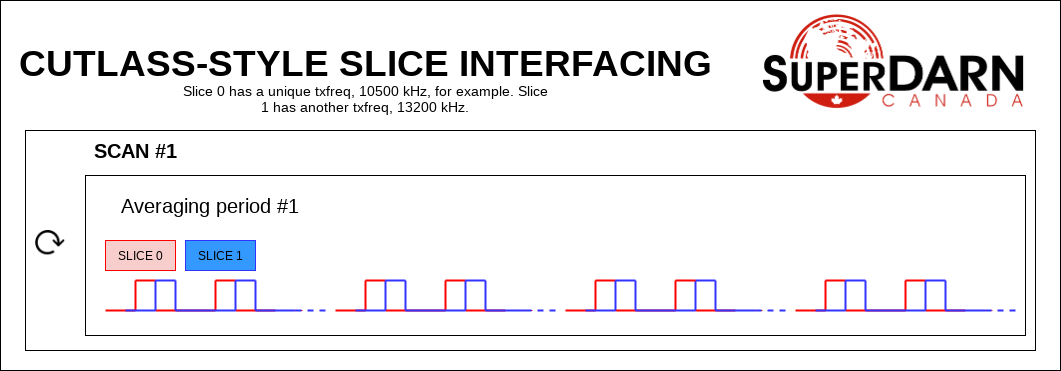
In a CUTLASS-style experiment, the pulse in the sequence is actually two pulses of differing transmit frequency. This is a ‘quasi’-simultaneous multi-frequency experiment where the frequency changes in the middle of the pulse. To build this experiment, two slices can be PULSE interfaced. The pulses from both slices are combined into a single set of transmitted samples for that sequence and samples received from those sequences are used for both slices (filtering the raw data separates the frequencies).
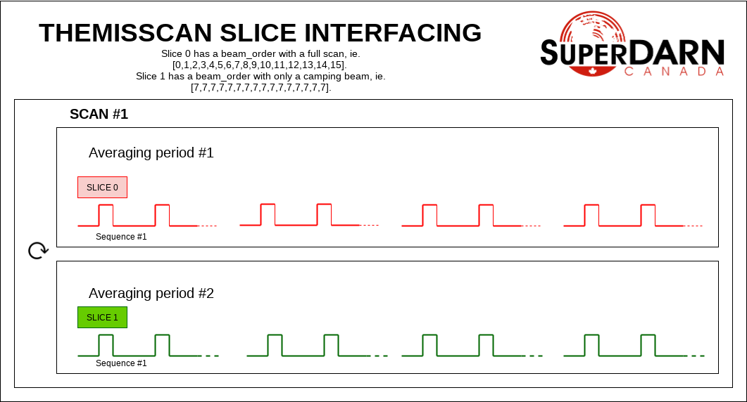
In a themisscan experiment, a single beam is interleaved with a full scan. The beam_order can be unique to different slices, and these slices could be INTTIME interfaced to separate the camping beam data from the full scan, if desired. With INTTIME interfacing, one averaging period of one slice will be followed by an averaging period of another, and so on. The averaging periods are interleaved. The resulting experiment runs beams 0, 7, 1, 7, etc.
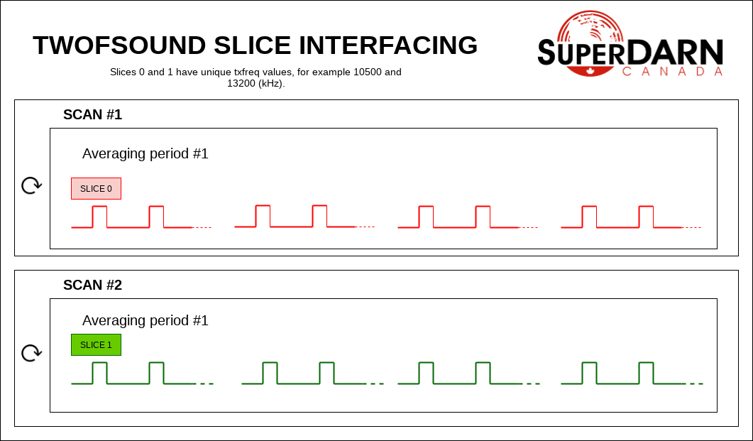
In a twofsound experiment, a full scan of one frequency is followed by a full scan of another frequency. The txfreq are unique between the slices. In this experiment, the slices are SCAN interfaced. A full scan of slice 0 runs followed by a full scan of slice 1, and then the process repeats.
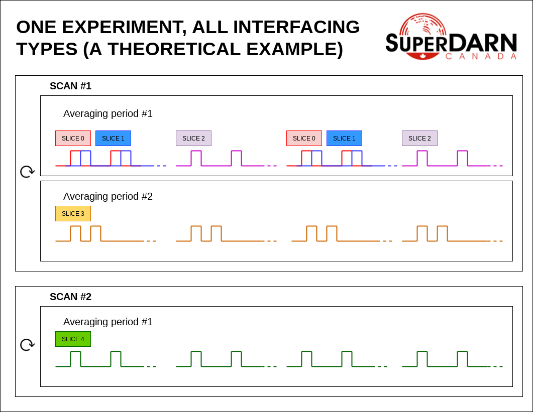
Here’s a theoretical example showing all types of interfacing. In this example, slices 0 and 1 are PULSE interfaced. Slices 0 and 2 are INTEGRATION interfaced. Slices 0 and 3 are INTTIME interfaced. Slices 0 and 4 are SCAN interfaced.
Writing an Experiment
All experiments must be written as their own class and must be built off of the built-in ExperimentPrototype class.
This means the ExperimentPrototype class must be imported at the start of the experiment file:
from experiments.experiment_prototype import ExperimentPrototype
Experiment-Wide Attributes
- cpid required
The only experiment-wide attribute that is required to be set by the user when initializing is the CPID, or control program identifier. This should be unique to the experiment. You will need to request this from your institution’s radar operator. You should clearly document the name of the experiment and some operating details that correspond to the CPID.
- output_rx_rate defaults
The sampling rate of the output data. The default is 10.0e3/3 Hz, or 3.333 kHz.
- rx_bandwidth defaults
The sampling rate of the USRPs (before decimation). The default is 5.0e6 Hz, or 5 MHz.
- tx_bandwidth defaults
The output sampling rate of the transmitted signal. The default is 5.0e6 Hz, or 5 MHz.
- txctrfreq defaults
The center frequency of the transmit chain. The default is 12000.0 kHz, or 12 MHz. Note that this is tuned so will be set to a quantized value, which in general is not exactly 12 MHz, and the value can be accessed by the user at this attribute after the experiment begins.
- rxctrfreq defaults
The center frequency of the receive chain. The default is 12000.0 kHz, or 12 MHz. Note that this is tuned so will be set to a quantized value, which in general is not exactly 12 MHz, and the value can be accessed by the user at this attribute after the experiment begins.
- decimation_scheme defaults
The decimation scheme for the experiment, provided by an instance of the class DecimationScheme. There is a default scheme specifically set for the default rates and center frequencies above.
- comment_string defaults
A comment string describing the experiment. It is highly encouraged to provide some description of the experiment for the output data files. The default is ‘’, or an empty string.
Below is an example of properly inheriting the prototype class and defining your own experiment:
class MyClass(ExperimentPrototype):

    def __init__(self):
        cpid = 123123  # this must be a unique id for your control program.
        super(MyClass, self).__init__(cpid,
            comment_string='My experiment explanation')
The experiment handler will create an instance of your experiment when your experiment is scheduled to start running. Your class is a child class of ExperimentPrototype and because of this, the parent class needs to be instantiated when the experiment is instantiated. This is important because the experiment_handler will build the scans required by your class in a way that is easily readable and iterable by the radar control program. This is done by methods that are set up in the ExperimentPrototype parent class.
The next step is to add slices to your experiment. An experiment is defined by the slices in the class, and how the slices interface. As mentioned above, slices are just dictionaries, with a preset list of keys available to define your experiment. The keys that can be used in the slice dictionary are described below.
Slice Keys
These are the keys that are set by the user when initializing a slice. Some are required, some can be defaulted, and some are set by the experiment and are read-only.
Slice Keys Required by the User
- pulse_sequence required
The pulse sequence timing, given in quantities of tau_spacing, for example normalscan = [0, 14, 22, 24, 27, 31, 42, 43].
- tau_spacing required
multi-pulse increment in us, Defines minimum space between pulses.
- pulse_len required
length of pulse in us. Range gate size is also determined by this.
- num_ranges required
Number of range gates.
- first_range required
distance to the first range gate, in km
- intt required or intn required
duration of an integration, in ms. (maximum)
- intn required or intt required
number of averages to make a single integration, only used if intt = None.
- beam_angle required
list of beam directions, in degrees off azimuth. Positive is E of N. The beam_angle list length = number of beams. Traditionally beams have been 3.24 degrees separated but we don’t refer to them as beam -19.64 degrees, we refer as beam 1, beam 2. Beam 0 will be the 0th element in the list, beam 1 will be the 1st, etc. These beam numbers are needed to write the beam_order list. This is like a mapping of beam number (list index) to beam direction off boresight. Typically you can use the radar’s common beam angle list. For example, at Saskatoon site the beam angles are a standard 16-beam list: [-26.25, -22.75, -19.25, -15.75, -12.25, -8.75,
-5.25, -1.75, 1.75, 5.25, 8.75, 12.25, 15.75, 19.25, 22.75, 26.25]
- beam_order required
beam numbers written in order of preference, one element in this list corresponds to one integration period. Can have lists within the list, resulting in multiple beams running simultaneously in the averaging period, so imaging. A beam number of 0 in this list gives us the direction of the 0th element in the beam_angle list. It is up to the writer to ensure their beam pattern makes sense. Typically beam_order is just in order (scanning W to E or E to W, ie. [0, 1, 2, 3, 4, 5, 6, 7, 8, 9, 10, 11, 12, 13, 14, 15]. You can list numbers multiple times in the beam_order list, for example [0, 1, 1, 2, 1] or use multiple beam numbers in a single integration time (example [[0, 1], [3, 4]], which would trigger an imaging integration. When we do imaging we will still have to quantize the directions we are looking in to certain beam directions.
- clrfrqrange required or txfreq or rxfreq required
range for clear frequency search, should be a list of length = 2, [min_freq, max_freq] in kHz. Not currently supported.
- txfreq required or clrfrqrange or rxfreq required
transmit frequency, in kHz. Note if you specify clrfrqrange it won’t be used.
- rxfreq required or clrfrqrange or txfreq required
receive frequency, in kHz. Note if you specify clrfrqrange or txfreq it won’t be used. Only necessary to specify if you want a receive-only slice.
Defaultable Slice Keys
- acf defaults
flag for rawacf and generation. The default is False. If True, the following fields are also used: - averaging_method (default ‘mean’) - xcf (default True if acf is True) - acfint (default True if acf is True) - lagtable (default built based on all possible pulse combos)
- acfint defaults
flag for interferometer autocorrelation data. The default is True if acf is True, otherwise False.
- averaging_method defaults
a string defining the type of averaging to be done. Current methods are ‘mean’ or ‘median’. The default is ‘mean’.
- comment defaults
a comment string that will be placed in the borealis files describing the slice. Defaults to empty string.
- lag_table defaults
used in acf calculations. It is a list of lags. Example of a lag: [24, 27] from 8-pulse normalscan. This defaults to a lagtable built by the pulse sequence provided. All combinations of pulses will be calculated, with both the first pulses and last pulses used for lag-0.
- pulse_phase_offset defaults
Allows phase shifting between pulses, enabling encoding of pulses. Default all zeros for all pulses in pulse_sequence.
- range_sep defaults
a calculated value from pulse_len. If already set, it will be overwritten to be the correct value determined by the pulse_len. This is the range gate separation, in azimuthal direction, in km.
- rx_int_antennas defaults
The antennas to receive on in interferometer array, default is all antennas given max number from config.
- rx_main_antennas defaults
The antennas to receive on in main array, default is all antennas given max number from config.
- scanbound defaults
A list of seconds past the minute for integration times in a scan to align to. Defaults to None, not required. If you set this, you will want to ensure that there is a slightly larger amount of time in the scan boundaries than the integration time set for the slice. For example, if you want to align integration times at the 3n second marks, you may want to have a set integration time of ~2.9s to ensure that the experiment will start on time. Typically 50ms difference will be enough. This is especially important for the last integration time in the scan, as the experiment will always wait for the next scan start boundary (potentially causing a minute of downtime). You could also just leave a small amount of downtime at the end of the scan.
- seqoffset defaults
offset in us that this slice’s sequence will begin at, after the start of the sequence. This is intended for PULSE interfacing, when you want multiple slice’s pulses in one sequence you can offset one slice’s sequence from the other by a certain time value so as to not run both frequencies in the same pulse, etc. Default is 0 offset.
- tx_antennas defaults
The antennas to transmit on, default is all main antennas given max number from config.
- xcf defaults
flag for cross-correlation data. The default is True if acf is True, otherwise False.
Read-only Slice Keys
- clrfrqflag read-only
A boolean flag to indicate that a clear frequency search will be done. Not currently supported.
- cpid read-only
The ID of the experiment, consistent with existing radar control programs. This is actually an experiment-wide attribute but is stored within the slice as well. This is provided by the user but not within the slice, instead when the experiment is initialized.
- rx_only read-only
A boolean flag to indicate that the slice doesn’t transmit, only receives.
- slice_id read-only
The ID of this slice object. An experiment can have multiple slices. This is not set by the user but instead set by the experiment automatically when the slice is added. Each slice id within an experiment is unique. When experiments start, the first slice_id will be 0 and incremented from there.
- slice_interfacing read-only
A dictionary of slice_id : interface_type for each sibling slice in the experiment at any given time.
Not currently supported and will be removed
- wavetype defaults
string for wavetype. The default is SINE. Not currently supported.
- iwavetable defaults
a list of numeric values to sample from. The default is None. Not currently supported but could be set up (with caution) for non-SINE. Not currently supported.
- qwavetable defaults
a list of numeric values to sample from. The default is None. Not currently supported but could be set up (with caution) for non-SINE. Not currently supported.
Experiment Example
An example of adding a slice to your experiment is as follows:
self.add_slice({  # slice_id will be 0, there is only one slice.
    "pulse_sequence": [0, 9, 12, 20, 22, 26, 27],
    "tau_spacing": tau_spacing,  # us
    "pulse_len": 300,  # us
    "num_ranges": 75,  # range gates
    "first_range": 180,  # first range gate, in km
    "intt": 3500,  # duration of an integration, in ms
    "beam_angle": [-26.25, -22.75, -19.25, -15.75, -12.25, -8.75,
                   -5.25, -1.75, 1.75, 5.25, 8.75, 12.25, 15.75, 19.25, 22.75,
                   26.25],
    "beam_order": [15, 14, 13, 12, 11, 10, 9, 8, 7, 6, 5, 4, 3, 2, 1, 0],
    "scanbound": [i * 3.5 for i in range(len(beams_to_use))], #1 min scan
    "txfreq" : 10500, #kHz
    "acf": True,
    "xcf": True,  # cross-correlation processing
    "acfint": True,  # interferometer acfs
})

self.add_slice(slice_1)
This slice would be assigned with slice_id = 0 if it’s the first slice added to the experiment. The experiment could also add another slice:
slice_2 = copy.deepcopy(slice_1)
slice_2['txfreq'] = 13200 #kHz
slice_2['comment'] = 'This is my second slice.'

self.add_slice(slice_2, interfacing_dict={0: 'SCAN'})
Notice that you must specify interfacing to an existing slice when you add a second or greater order slice to the experiment. To see the types of interfacing that can be used, see above section ‘Interfacing Types Between Slices’.
This experiment is very similar to the twofsound experiment. To see examples of common experiments, look at experiments package.